2. CO2/N2 Unary Example
In this example, we fit temperature-dependent unary data from [PXSL14].
2.1. Initialization
We first load the necessary packages
>>> import pyomo.environ as pyo
>>> import matplotlib.pyplot as plt
>>> import pandas as pd
>>> from isotherm_models.unaryisotherm import LangmuirUnary
2.2. CO2
We first get the data from the data file
>>> data = pd.read_csv('data_sets/CO2_BEA.csv')
Using pandas, we can easily take a peek at the data we have input from our .csv file
>>> data.head()
    P [atm]  Q [mmol/g]  T [K] adsorbate
0  0.029814    0.096491  273.0       CO2
1  0.055856    0.175439  273.0       CO2
2  0.109177    0.328947  273.0       CO2
3  0.246821    0.719298  273.0       CO2
4  0.313781    0.903509  273.0       CO2
Before solving the model, we convert the partial pressures to si units
>>> P_i = data['P [atm]']*101325 # convert to Pa -- si units
so that we can create the model
>>> co2_model = LangmuirUnary(P_i, data['Q [mmol/g]'], data['T [K]'], name='CO2')
and solve it
>>> co2_model.solve()
We then take a look at the results
>>> co2_model.get_R2_pyomo()
0.99796
>>> co2_model.get_objective()
0.007229102
>>> co2_model.dH_i.display()
dH_i : Size=1
    Key  : Value
    None : -20780.90809523844
>>> co2_model.q_mi.display()
q_mi : Size=1
    Key  : Value
    None : 8.95582798469325
>>> co2_model.k_i_inf.display()
k_i_inf : Size=1
    Key  : Value
    None : 3.8656918601559114e-10
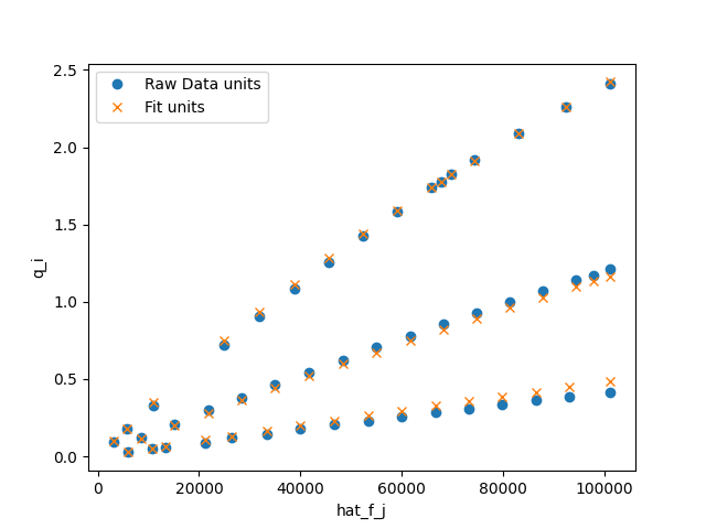
And save the results to a file
>>> fig = plt.figure()
>>> fig, ax = co2_model.plot_unary(fig=fig)
>>> _ = ax.legend()
>>> fig.savefig('docs/source/CO2_example.png')
which looks like
2.3. N2
We repeat a similar approach for the N2 isotherms, first formatting the data for input to the model
>>> data = pd.read_csv('data_sets/N2_BEA.csv')
Using pandas, we can easily take a peek at the data we have input from our .csv file
>>> data.head()
    P [atm]  Q [mmol/g]  T [K] adsorbate
0  0.525470    0.070175  303.0        N2
1  0.592387    0.078947  303.0        N2
2  0.656824    0.083333  303.0        N2
3  0.722502    0.092105  303.0        N2
4  0.788179    0.100877  303.0        N2
Before solving the model, we convert the partial pressures to si units
>>> P_i = data['P [atm]']*101325 # convert to Pa -- si units
Instantiating (creating) the model
>>> n2_model = LangmuirUnary(P_i, data['Q [mmol/g]'], data['T [K]'], name='N2')
Solving it
>>> n2_model.solve()
We then take a look at the results
>>> n2_model.get_R2_pyomo()
0.99262
>>> n2_model.get_objective()
0.00194249
>>> n2_model.dH_i.display()
dH_i : Size=1
    Key  : Value
    None : -12557.526993112784
>>> n2_model.q_mi.display()
q_mi : Size=1
    Key  : Value
    None : 0.45280441671269905
>>> n2_model.k_i_inf.display()
k_i_inf : Size=1
    Key  : Value
    None : 2.412336128388879e-08
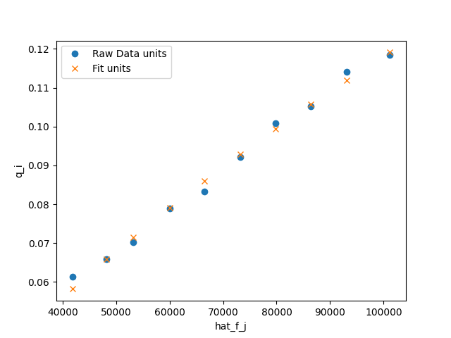
And save the results to a file
>>> fig = plt.figure()
>>> fig, ax = n2_model.plot_unary(fig=fig)
>>> _ = ax.legend()
>>> fig.savefig('docs/source/N2_example.png')
which looks like
2.4. Comparison to scipy
>>> import numpy as np
>>> popt, pcov = co2_model.solve_scipy()
>>> popt
array([  3.71939309, -10.14817759,  -7.28715595])
>>> popt - np.array(list(map(pyo.value, [co2_model.q_mi_star, co2_model.A_i, co2_model.H_i_star])))
array([3.28355311e-05, 3.67969745e-05, 3.88858220e-05])